Tutorial

Before running the code from this tutorial, we recommend that you set up your environment by following the instructions in the getting started section of the documentation.

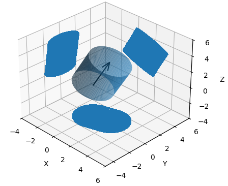
The Cylinder class is used to represent the 3-D cylinders that make up a QSM. The most important function of these Cylinder objects is their ability to return data regarding the projections onto the XY, XZ and YZ planes.

  myCyl = Cylinder(
    cyl_id=1.0,
    x=[3, 6],
    y=[2, 4],
    z=[6, 12],
    radius=2.0,
    length=0.064433,
    branch_order=0.0,
    branch_id=0.0,
    volume=0.010021,
    parent_id=0.0,
    reverse_branch_order=32.0,
    segment_id=0.0,
  )
  fig = myCyl.draw_3D(show=False, draw_projections=True)

The Cylinder Collection class is a data class consisting of multiple cylinders and related metrics. Cylinder Collections almost always represent [QSMs](https://canopyhydrodynamics.readthedocs.io/en/latest/qsms.html#) or parts of a QSM and are meant to help users explore these QSMs. Below, we demonstrate how one might create a cylinder collection using cylinder data (e.g. QSM data) stored in a CSV file and how the afforementioned concept of projections can be used to visualize the data in a variety of ways. Note: the tree chosen for the below is intentionally small to make the visualization easier to understand.

# Creating a CylinderCollection object
myCollection = CylinderCollection()

# The below file is one of our several testing files featuring only
# the trunk of a tree and one of its branches
myCollection.from_csv("charlie_brown.csv")

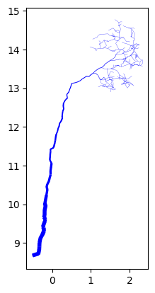
# plot the tree as seen from the 'front'
myCollection.draw("XZ")

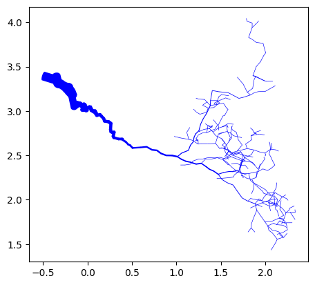
# plot the tree as seen from above
myCollection.draw("XY")

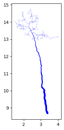
# plot the tree as seen from the 'side'
myCollection.draw("YZ")

XZ Projection

XY Projection

YZ Projection

Compared to a QSM, CylinderCollections have additional structure in the form of a digraph model. These digraph models represent the direction water flows along the branches of the modeled tree and are used in the ‘find_flow_components’ and ‘calculate_flows’ function to characterize the flow of water through the canopy. The below code, continuing from the above demonstrates the use of these functions.

# creating the digraph model
myCollection.initialize_digraph_from()

# Identifying the flows to which each cyl belongs
myCollection.find_flow_components()

# Calculating the propreties of each flow
myCollection.calculate_flows()

# Print out recommend flow characteristics
print(myCollection.flows)

num_cylinders	projected_area	surface_area	angle_sum	volume	sa_to_vol	drip_node_id	drip_node_loc
162.0	0.345	1.167	111.92	0.019	82717.985	0.0	(-0.5, 3.4, 8.7)
18	0.005	0.021	10.275	0.0	14370.354	232	(1.9, 2.2, 13.9)
13	0.004	0.015	7.718	0.0	11229.764	360	(1.8, 2.6, 13.6)
24	0.008	0.032	1.697	0.0	18378.751	515	(1.5, 2.8, 12.9)
…	…	…	…	…	…	…	…

What you see above is a sample of the flow characteristics calculated for the ‘charlie_brown’ tree. The first flow listed is, as is the convention in canoPyHydro, the tree’s stemflow and the others are the throughfall flows. The ‘drip_node_loc’ column lists the x,y,z coordinates of the node of the afformentioned graph to which water intercepted by the flow’s cylinders is directed. The various geometric characteristics give a sense of the size and shape of the flow’s cylinders (or ‘canopy drainage area’).

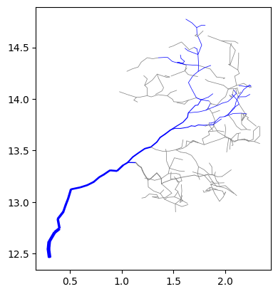
The draw function also allows for a variety of different overlays, filtering and highlighting. To demonstrate this briefly, we will show below how this filtering can be used in a variety of ways, including highlighting the various flows mentioned above. For more information on the CylinderCollection class, please refer to the documentation.

# Plot the entire tree with stem flow highlighted
myCollection.draw("XZ", highlight_lambda=lambda:is_stem)

# Plot the interesting portion of the tree with stem flow highlighted
myCollection.draw("XZ",
                  highlight_lambda=lambda:is_stem,
                  filter_lambda=lambda: cyl_id>100)

# Adding drip points to the above mentioned plot
myCollection.draw("XZ",
                  highlight_lambda=lambda:is_stem,
                  filter_lambda=lambda: cyl_id>100,
                  include_drips=True)

Plot of the entire tree

Same as left but zoomed in

Adding locations of drip points

The final bit of functionality we will review today is the ability to create concave hulls around groups of cylinders in a CylinderCollection. This is done using the ‘watershed_boundary’ function. The below code demonstrates how this function can be used to find a concave hull around the entire tree, or a portion of the tree. Note that a new, more robist example tree is used

# Reading in the tree data and finding flows
myCollection = CylinderCollection()
myCollection.from_csv("example_tree.csv")
myCollection.project_cylinders("XY")
myCollection.initialize_digraph_from()
myCollection.find_flow_components()
myCollection.calculate_flows()

#drawing the tree for reference
myCollection.draw("XY", save=True, file_name_ext="read_me_alpha")

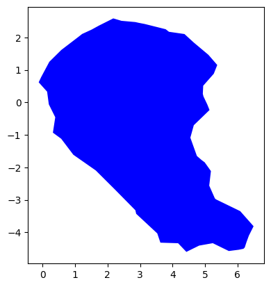
# Drawing the whole canopy boundary
myCollection.watershed_boundary(plane = 'XY', draw=True)

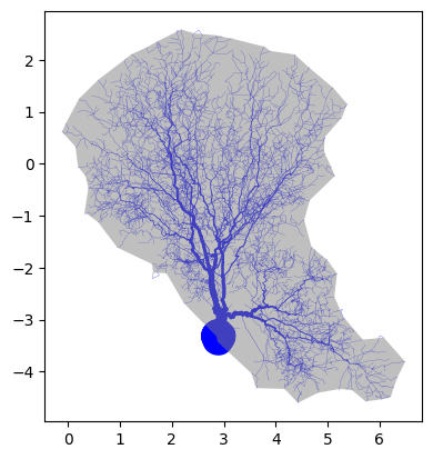
# Drawing the canopy boundary and tree together
myCollection.draw("XY",
                  include_alpha_shape=True)

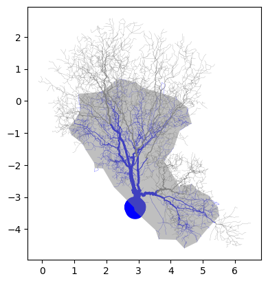
# Drawing a tighter fitting alpha shape
myCollection.watershed_boundary(plane = 'XY',
                                curvature_alpha=2,
                                draw=True)
myCollection.draw("XY",
                  include_alpha_shape=True)

# Drawing the stem flow watershed boundary
# with stemflow cylinders highlighted
myCollection.watershed_boundary(plane = 'XY',
                                curvature_alpha=2,
                                filter_lambda=lambda: is_stem)
myCollection.draw("XY",
                  include_alpha_shape=True,
                  highlight_lambda=lambda: is_stem)

Entire canopy hull alone

Hull overlaid on the canopy

A tighter fitting hull

The stem flow boundary hull