Flow Identification
[10]:
# For the purposes of this tutorial, we will turn off logging
import logging
import os
logger = logging.getLogger()
logger.setLevel(logging.CRITICAL)

# Determines where configuration file is located
# # file contains directory info and model input settings
config_file = os.environ[
    "CANOPYHYDRO_CONFIG"
] = f"{os.getcwd()}/canopyhydro_config.toml"
log_config = os.environ["CANOPYHYDRO_LOG_CONFIG"] = f"{os.getcwd()}/docs/source/examples/logging_config.yml"
print(os.getcwd())
print(os.environ["CANOPYHYDRO_LOG_CONFIG"])
/code/code/canopyHydrodynamics
/code/code/canopyHydrodynamics/docs/source/examples/logging_config.yml
Graph Models
[1]:
# How Graphs are initialized

import os

os.environ["CANOPYHYDRO_CONFIG"] = "./canopyhydro_config.toml"
from src.canopyhydro.CylinderCollection import CylinderCollection

# Initializing a CylinderCollection object
myCollection = CylinderCollection()

# Converting a specified file to a CylinderCollection object
myCollection.from_csv("5_SmallTree.csv")

# Requesting an plot of the tree projected onto the XY plane (birds-eye view)
myCollection.project_cylinders("XY")

# creating the digraph model
myCollection.initialize_digraph_from()
2024.10.14 21:01:20.326 |MainThread | INFO | CylinderCollection.py:291 - from_csv() | model - Processing <_io.TextIOWrapper name='./data/input/5_SmallTree.csv' mode='r' encoding='UTF-8'>
2024.10.14 21:01:20.361 |MainThread | INFO | CylinderCollection.py:320 - from_csv() | model - ./data/input/5_SmallTree.csv initialized with 517 cylinders
2024.10.14 21:01:20.363 |MainThread | INFO | CylinderCollection.py:335 - project_cylinders() | model - Projection into XY axis begun for file 5_SmallTree.csv
2024.10.14 21:01:22.259 |MainThread | INFO | CylinderCollection.py:344 - project_cylinders() | model - Projection into XY axis complete for file 5_SmallTree.csv
These graphs are instances of ‘DiGraph’ objects from the ‘networkx’ package. For more information regarding their capabilities, reffer to the afforementioned linked documentation.
For our purposes, you just need to know that the edges of these graphs correspond to the cylinders in a CylinderCollection. So, when the ‘find_flow_components’ function traverses a graph, it is akin to walking along the branches of the tree.
[8]:
# See how cylinder 0 (the base of the tree) correlates
#  to edge 0 in our graph
print(myCollection.graph.edges(1,data=True))
print(myCollection.cylinders[1])
[(1, 0, {'cylinder': Cylinder( cyl_id=1.0, x=[-0.299115 -0.638138], y=[2.537844 2.995146], z=[-0.552    -0.354452], radius=0.531411, length=0.602566, branch_order=0.0, branch_id=0.0, volume=0.534583, parent_id=0.0, reverse_branch_order=67.0, segment_id=0.0})]
Cylinder( cyl_id=1.0, x=[-0.299115 -0.638138], y=[2.537844 2.995146], z=[-0.552    -0.354452], radius=0.531411, length=0.602566, branch_order=0.0, branch_id=0.0, volume=0.534583, parent_id=0.0, reverse_branch_order=67.0, segment_id=0.0
Each of the edges in the graph, also have a direction, depending on their angle in space. In particular, each edge is directed in the direction in which intercepted water is presumed to flow.
During traversal, each edge may only be traversed in the direction it has been assigned. For example, every cylinder in the stem is oriented towards its base so, just as is the case with water, the only direction in which we can traverse from trunk edge to trunk edge is downward.
[9]:
# Looking at the cylinders accessable from our stem cylinders (i.e. their neighbors)
print('The following cylinders are accessable from cylinder 5: ')
print([x for x in myCollection.graph.neighbors(5)])
print('The following cylinders are accessable from cylinder 4: ')
print([x for x in myCollection.graph.neighbors(4)])
print('The following cylinders are accessable from cylinder 3: ')
print([x for x in myCollection.graph.neighbors(3)])
print('The following cylinders are accessable from cylinder 2: ')
print([x for x in myCollection.graph.neighbors(2)])
print('The following cylinders are accessable from cylinder 1: ')
print([x for x in myCollection.graph.neighbors(1)])
The following cylinders are accessable from cylinder 5:
[4]
The following cylinders are accessable from cylinder 4:
[3]
The following cylinders are accessable from cylinder 3:
[2]
The following cylinders are accessable from cylinder 2:
[1]
The following cylinders are accessable from cylinder 1:
[0]
Finding Flows
This traversal (indeed much of anything at all to do with these graphs), is handled behind the scenes.
The code below shows how a user can call ‘find_flow_components’ to trigger the use of the collections graph and therefore identify the paths water takes - the flows - in the tree canopy
[5]:
# Finding the flows in the canopy

import os

os.environ["CANOPYHYDRO_CONFIG"] = "./canopyhydro_config.toml"
from canopyhydro.CylinderCollection import CylinderCollection

# Initializing a CylinderCollection object
myCollection = CylinderCollection()

# Converting a specified file to a CylinderCollection object
myCollection.from_csv("5_SmallTree.csv")

# Requesting an plot of the tree projected onto the XY plane (birds-eye view)
myCollection.project_cylinders("XY")

# creating the digraph model
myCollection.initialize_digraph_from()

# Traversing the graph, determining the fate of the water
# intercepted by each cylinder
myCollection.find_flow_components()

# For each of the possible destinations for said water,
#   summing the volume, area, etc of the contributing cylinders
myCollection.calculate_flows()

for i in range(20):
    print(myCollection.flows[i])
2024.10.14 21:04:19.312 |MainThread | INFO | CylinderCollection.py:291 - from_csv() | model - Processing <_io.TextIOWrapper name='./data/input/5_SmallTree.csv' mode='r' encoding='UTF-8'>
2024.10.14 21:04:19.379 |MainThread | INFO | CylinderCollection.py:320 - from_csv() | model - ./data/input/5_SmallTree.csv initialized with 517 cylinders
2024.10.14 21:04:19.383 |MainThread | INFO | CylinderCollection.py:335 - project_cylinders() | model - Projection into XY axis begun for file 5_SmallTree.csv
2024.10.14 21:04:21.355 |MainThread | INFO | CylinderCollection.py:344 - project_cylinders() | model - Projection into XY axis complete for file 5_SmallTree.csv
2024.10.14 21:04:21.687 |MainThread | INFO | CylinderCollection.py:769 - find_flow_components() | model - 5_SmallTree.csv found to have 70 drip components
reached_End of find flows
Flow(num_cylinders=216.0, projected_area=16.51706021532694, surface_area=19.495074988550606, angle_sum=180.03288665020426, volume=3.9062960000000007, sa_to_vol=83646.49652248439, drip_node_id=0.0, drip_node_loc=(-0.299115, 2.537844, -0.598273))
Flow(num_cylinders=2, projected_area=0.0005597565466076131, surface_area=0.001924052712727801, angle_sum=-0.8861661864942612, volume=2e-06, sa_to_vol=1924.052712727801, drip_node_id=148, drip_node_loc=(1.736771, 2.700067, 14.216883))
Flow(num_cylinders=4, projected_area=0.0012679984136685896, surface_area=0.0043875954238933096, angle_sum=-1.1103646559240672, volume=4.9999999999999996e-06, sa_to_vol=3681.4517891642977, drip_node_id=150, drip_node_loc=(1.476039, 2.744678, 14.221036))
Flow(num_cylinders=1, projected_area=0.00026175097799692134, surface_area=0.0008268043545717619, angle_sum=0.20259148846207123, volume=1e-06, sa_to_vol=826.8043545717619, drip_node_id=159, drip_node_loc=(1.298384, 2.459679, 14.389457))
Flow(num_cylinders=3, projected_area=0.0008824774277666259, surface_area=0.0032463019367339413, angle_sum=-1.7087376025874943, volume=3e-06, sa_to_vol=3246.3019367339416, drip_node_id=164, drip_node_loc=(1.047176, 2.391643, 14.266511))
Flow(num_cylinders=2, projected_area=0.0006600186476422296, surface_area=0.0023746199311056493, angle_sum=0.534393748750537, volume=3e-06, sa_to_vol=1719.5271769974715, drip_node_id=175, drip_node_loc=(1.730164, 2.302889, 14.604732))
Flow(num_cylinders=2, projected_area=0.0004876054032408554, surface_area=0.001917581031861406, angle_sum=1.1425108485836808, volume=3e-06, sa_to_vol=1179.8879529087187, drip_node_id=179, drip_node_loc=(1.652252, 2.280224, 14.47647))
Flow(num_cylinders=1, projected_area=0.00041651108754572896, surface_area=0.0014212408085207547, angle_sum=-0.4465420656788475, volume=2e-06, sa_to_vol=710.6204042603774, drip_node_id=183, drip_node_loc=(1.455036, 2.239273, 14.49977))
Flow(num_cylinders=2, projected_area=0.0012733736410329834, surface_area=0.004064592575214475, angle_sum=-0.3665923044681696, volume=4.9999999999999996e-06, sa_to_vol=1666.127955868079, drip_node_id=187, drip_node_loc=(1.917529, 2.347151, 14.212591))
Flow(num_cylinders=0, projected_area=0.0, surface_area=0.0, angle_sum=0.0, volume=0.0, sa_to_vol=0.0, drip_node_id=189, drip_node_loc=(1.984224, 2.47876, 14.194845))
Flow(num_cylinders=6, projected_area=0.0022330283517565724, surface_area=0.007333246943678708, angle_sum=2.127804515876493, volume=9.999999999999999e-06, sa_to_vol=4446.06831715825, drip_node_id=193, drip_node_loc=(1.583993, 2.563848, 13.968024))
Flow(num_cylinders=1, projected_area=0.00020343043979622444, surface_area=0.0006478435290600194, angle_sum=0.2846026246124941, volume=1e-06, sa_to_vol=647.8435290600194, drip_node_id=198, drip_node_loc=(1.284843, 2.628993, 14.019867))
Flow(num_cylinders=3, projected_area=0.0007860084747630203, surface_area=0.003617512524682111, angle_sum=-2.5833501908977685, volume=4.9999999999999996e-06, sa_to_vol=2085.8447343876755, drip_node_id=208, drip_node_loc=(1.325472, 2.856421, 14.043133))
Flow(num_cylinders=2, projected_area=0.0006471769977986668, surface_area=0.0020395847825635657, angle_sum=0.26090730746353386, volume=2e-06, sa_to_vol=2039.584782563566, drip_node_id=209, drip_node_loc=(1.435887, 2.797216, 14.208758))
Flow(num_cylinders=8, projected_area=0.0017034251569991014, surface_area=0.007463890074178239, angle_sum=5.354426428330182, volume=8.999999999999999e-06, sa_to_vol=6831.314685414667, drip_node_id=214, drip_node_loc=(1.178362, 2.670965, 14.017909))
Flow(num_cylinders=3, projected_area=0.0012809041391582444, surface_area=0.004173213141212342, angle_sum=0.3207042500076585, volume=6e-06, sa_to_vol=2086.606570606171, drip_node_id=219, drip_node_loc=(1.152153, 2.815179, 13.969726))
Flow(num_cylinders=2, projected_area=0.0008570559793830896, surface_area=0.0027383692365015432, angle_sum=-0.10344238545184348, volume=4e-06, sa_to_vol=1369.1846182507718, drip_node_id=222, drip_node_loc=(1.607588, 2.540239, 13.949144))
Flow(num_cylinders=0, projected_area=0.0, surface_area=0.0, angle_sum=0.0, volume=0.0, sa_to_vol=0.0, drip_node_id=227, drip_node_loc=(1.868195, 2.555224, 13.948772))
Flow(num_cylinders=18, projected_area=0.005313162793692856, surface_area=0.021339283807471944, angle_sum=10.274852917465788, volume=2.6e-05, sa_to_vol=14370.354273860652, drip_node_id=232, drip_node_loc=(1.920238, 2.162247, 13.938462))
Flow(num_cylinders=7, projected_area=0.0029795345832851253, surface_area=0.013586461456943049, angle_sum=4.695171005225782, volume=1.8e-05, sa_to_vol=5378.31106616918, drip_node_id=242, drip_node_loc=(2.047486, 1.966398, 14.326444))
For more information on how the statistics calculated by ‘calculate_flows’ are used, see statistics
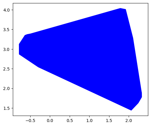
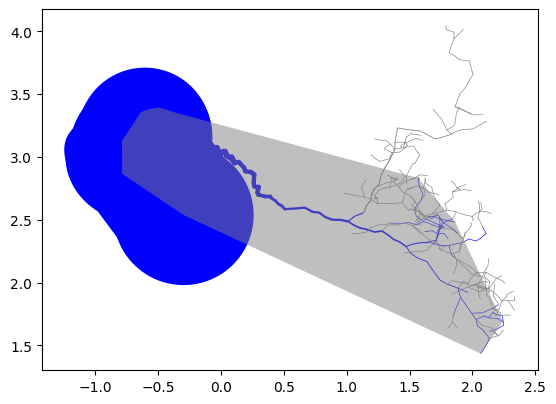
Figures
The usage of the ‘watershed_boundary’ function is coverd in the Concave Hulls and Watersheds example doc, so we will not go too into depth on them here.
[10]:
#Figures using 'is_stem'
#plotting the entire watershed boundary
whole_tree_hull,_ = myCollection.watershed_boundary(
plane="XY",
curvature_alpha=0.15,
draw=True,
)
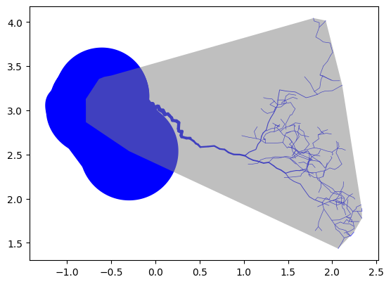
# plotting the whole tree boundary with the tree
# with stemflow branches highlighted
myCollection.draw(
"XY",
include_alpha_shape=True
)
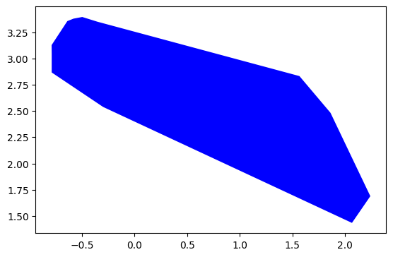
# plotting the boundary of the stemflow generating portion alone
stem_flow_hull,_ = myCollection.watershed_boundary(
plane="XY",
curvature_alpha=0.15,
filter_lambda=lambda: is_stem ,
draw=True,
)
# plotting the stemflow boundary with the tree
# with stemflow branches highlighted
myCollection.draw(
"XY",
include_alpha_shape=True,
highlight_lambda=lambda: is_stem
)
2024.10.14 18:32:37.020 |MainThread | INFO | geometry.py:563 - draw_cyls() | model - Plotting cylinder collection
2024.10.14 18:32:37.140 |MainThread | INFO | CylinderCollection.py:403 - draw() | model - 517 cylinders matched criteria
overlay [<POLYGON ((-0.497 3.394, 1.788 4.044, 1.927 4.016, 2.113 3.284, 2.327 1.93, ...>]
2024.10.14 18:32:37.143 |MainThread | INFO | geometry.py:563 - draw_cyls() | model - Plotting cylinder collection
2024.10.14 18:32:37.437 |MainThread | ERROR | geometry.py:591 - draw_cyls() | model - Overlay must be a Polygon, a list of Polygons or coordinate list
2024.10.14 18:32:37.525 |MainThread | INFO | geometry.py:563 - draw_cyls() | model - Plotting cylinder collection
2024.10.14 18:32:37.617 |MainThread | INFO | CylinderCollection.py:403 - draw() | model - 517 cylinders matched criteria
overlay [<POLYGON ((-0.639 3.355, -0.581 3.378, -0.497 3.394, -0.353 3.349, 1.567 2.8...>]
2024.10.14 18:32:37.621 |MainThread | INFO | geometry.py:563 - draw_cyls() | model - Plotting cylinder collection
2024.10.14 18:32:38.002 |MainThread | ERROR | geometry.py:591 - draw_cyls() | model - Overlay must be a Polygon, a list of Polygons or coordinate list
[10]:
<Axes: >
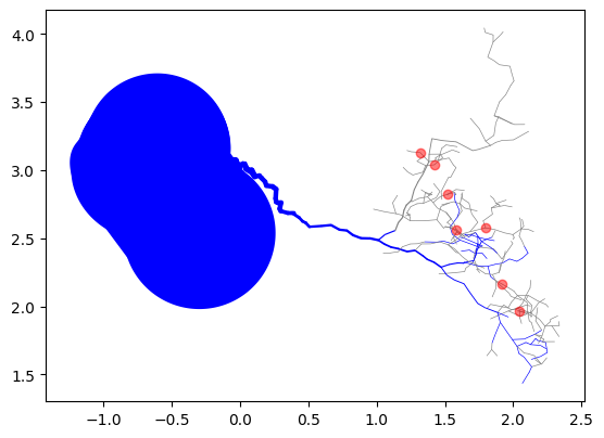
Once flows have been found for a cylinderCollection, the draw funtion can also access the locations of the drip points and overlay them onto a figure
[11]:
# Adding drip points to and XY view of myCollection
myCollection.draw(
    "XY",
    highlight_lambda=lambda: is_stem,
    include_drips=True,
)
2024.10.14 18:32:56.455 |MainThread | INFO | CylinderCollection.py:403 - draw() | model - 517 cylinders matched criteria
2024.10.14 18:32:56.461 |MainThread | WARNING | CylinderCollection.py:433 - draw() | model - No drip point locations found, running set_drip_points
overlay [[[1.583993, 1.920238, 2.047486, 1.797333, 1.421225, 1.317245, 1.520497], [2.563848, 2.162247, 1.966398, 2.576308, 3.038762, 3.130179, 2.822484]]]
2024.10.14 18:32:56.468 |MainThread | INFO | geometry.py:563 - draw_cyls() | model - Plotting cylinder collection
[11]:
<Axes: >